A Note on the Dimension of Random Vectors in End-to-End Differentiable Systems
If you are interested in a quick read, you may skip the introduction.
Introduction
Although the primary application of libraries such as TensorFlow and PyTorch is deep learning, they are also excellent for optimizations in the overlapping framework of differentiable programming. They allow composing functions that are differentiable into larger systems that are end-to-end differentiable, and by using automatic differentiation they make gradient-based optimization easier.
One setting which comes up sometimes is the optimization of the parameters of a subsystem which is part of a larger stochastic system. Here is a typical example, where system \(A\) with parameters \(\theta\) feeds system \(B\).
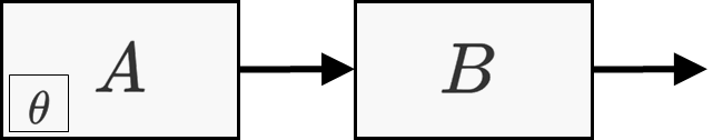
The output of system \(B\) is differentiable with respect to its input from system \(A\), and the output of system \(A\) is differentiable with respect to its parameters \(\theta\). System \(B\) stochastic, in the sense that its output depends not only on its input but also on the results of drawing some random numbers.
An example for such a system is \(A\) being some open-loop controller that controls a physical system \(B\) which is not deterministic. Actually, system \(B\) in this case is a stochastic differentiable simulation of a real system, implemented in, e.g. PyTorch. As a more concrete example, \(A\) can represent the impulses produced by a motor in some robot, and \(B\) is a physics simulation of how the robot’s arms respond to the impulse.
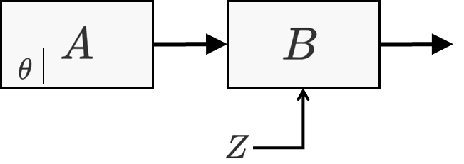
We said that \(B\) is a stochastic function. It is actually useful to separate the stochastic and deterministic elements of \(B\). Since stochasticity is manifested by sampling from a random number generator, we will collectively denote all the random numbers as \(Z\), and we will view \(Z\) as being an additional input to \(B\). Now, \(B\) is viewed as deterministic with a random input \(Z\) (in addition to the input from \(A\)).
\(B\) can take many forms. For example, it can be a neural network, or it can be a MCMC-based simulator, or it can be an integrator of equations of motions, or anything else, as long as it is differentiable with respect to its input from \(A\), and as long as all of its sources of randomness are bundled into \(Z\).
Henceforth, we will assume that \(Z\) is a standard normal random vector of dimension \(d\): \(Z\sim\mathcal{N}(0,I_{d\times d})\). And we will write the output of the system as \(B(A_\theta,Z)\). This should be a differentiable function with respect to \(\theta\), and the gradient with respect to \(\theta\) is typically calculated using automatic differentiation.
The goal is to minimize some objective function \(f\) applied on \(B\)’s output. (\(f\) too needs to be differentiable): \(f(B(A_\theta,Z))\). Since this is random, what we actually want to minimize is \(g(\theta)=\mathbb{E}[f(B(A_\theta,Z))]\). Gradient-based optimization can be used, but it needs to be stochastic gradient descent (SGD; or one of its variants). In other words, on each iteration, a batch of \(Z\) values is sampled from \(Z\sim\mathcal{N}(0,I)\), then the gradient \(\nabla_\theta f(B(A_\theta,Z))\) is calculated for each \(Z\) in the batch, and these gradients are averaged over the batch. This serves as the unbiased estimate of the gradient of \(g(\theta)\) and is used for updating the parameters \(\theta\).
The gradient estimate is unbiased, but it has variance whose source is \(Z\). The smaller the variance, the better the gradient estimation is, the more efficient the optimization is. (note: when doing SGD for DL, it is often argued that the variance is beneficial as it improves the generalization performance of the model; but here we are in a different context. Also, the argument that the variance is helpful for escaping local minima might be valid, but even with zero variance it is easy to get the same effect by simply adding noise with any desired variance). The variance will decrease the larger the batch size, at the expense of more computations done per batch.
To simplify the notation a bit, we will define from now on \(C(\theta,Z)=B(A_\theta,Z)\).
In the following, a heuristic argument will be made as for the dependence of the variance on the dimensionality of \(Z\).
The Argument
(The following is a rough heuristic argument. To make it precise, several assumptions need to be made, about continuity etc.).
We have \(Z\) a random vector of dimension \(d\), and we want to find the optimal \(\theta\) of \(g(\theta)=\mathbb{E}[f(C(\theta,Z))]\) using SGD, where \(f\) is some objective function applied on the output of \(C\). For a fixed \(\theta\), we will denote by \(m\) the dimension of the image of \(Z\rightarrow C(\theta, Z)\), viewed as some manifold (so that \(m\) is not the size of \(C(\theta,Z)\), it is dimension of the hypersurface which is the image of the function).
When doing backpropagation on \(g(\theta)\), one of the steps is to calculate the gradient of \(C\). Let \(X=C(\theta, Z)\) and \(Y=\nabla_\theta C(\theta,Z)\) be two random variables. \(X\) is actually a random vector and \(Y\) is a random matrix.
From the law of total variance, (applied elementwise), we have:
\(\text{Var}[\nabla_\theta C(\theta,Z)]=\text{Var}(Y)=\mathbb{E}[\text{Var}(Y\vert X)]+\text{Var}[\mathbb{E}(Y\vert X)]\) .
Now, let’s look at two cases. In the first case, \(d \approx m\). In this case, the mapping \(Z\rightarrow C(\theta,Z)\) is likely to be one-to-one, at least to a high degree. Therefore, in the law of total variance, the first term will approximately vanish: given the value of \(X\) , the value of \(Z\) is determined, and therefore the value of \(Y\) is determined, and the variance becomes zero. Thus, in this case we have \(\text{Var}(Y)\approx\text{Var}[\mathbb{E}(Y\vert X)]\). Moreover, since \(Y\) is determined from \(X\), we can write \(Y\) as a function of \(X\): \(\ \ Y=Y(X)\) and we get \(\text{Var}(Y)\approx \text{Var}(Y(X))\) . Notice that this shows that the variance of \(\nabla_\theta C(\theta,Z)\) is only due to the variance of \(C(\theta,Z)\). This variance is irreducible (in the sense that if a real system was used instead of its perfect simulator \(C\), we would get the same variance).
The second case, \(d > m\). (The case \(d < m\) cannot really exist, assuming the mapping \(Z\rightarrow C(\theta, Z)\) is sufficiently regular…). This means that the mapping is many-to-one. Hence, the first term cannot be neglected. This means that we get an additional source of variance, representing the fact that a single value of \(C(\theta,Z)\) can be represented using multiple values of \(Z\).
The conclusion is that, to have the smallest variance in the gradient estimator, we should choose the \(Z\) with smallest size possible.
If we have freedom in designing the dependence of the function \(C(\theta,Z )\) on \(Z\), with the constraint that the function gives some output distribution, we should reduce the size of \(Z\) as much as possible consistent with being able to satisfy the constraint. This will give smallest variance in the SGD gradient estimator, and will therefore allow faster convergence.