Visualizing Policies of Soft Actor Critic

The code associated with this post is here.

In reinforcement learning (RL), the typical goal is to find a policy \(\pi(a \vert s)\), that is, a probability distribution for an agent’s action \(a\) given an observed state \(s\), such that the mean total reward \(J(\pi)\) is maximal:

\(\tau\) is a trajectory defined as a sequence of states and actions \((s_0,a_0),(s_1,a_1),...,(s_t,a_t),...\), and the notation \(\tau\sim\pi\) means that the trajectory is sampled using the policy \(\pi\) and the state transition function (we assume the dynamics to be Markovian). \(r(s_t,a_t)\) is the reward (which can also be random). If the length of trajectories is unbounded, we also need a discount factor, but we ignore this for now.

The policy \(\pi(a \vert s)\) represents a probability distribution. However, among all of the policies \(\pi\) that maximize \(J(\pi)\), at least some of them will be deterministic (meaning that given the state, the action is non-random). It can be shown (I think) that if \(\pi_1\) is a maximizer of \(J(\pi)\), and we modify \(\pi_1\) to be deterministic (by shifting all the probability mass \(\pi_1(a \vert s)\) to a single action \(a\) which has positive probability under \(\pi_1(a \vert s)\)), then the modified policy will also maximize \(J(\pi)\). But this does not mean that all maximizers are deterministic! However, to have a non-deterministic maximizer usually means that there is some exact symmetry of the environment, or that some parts of the action space do not affect the environment. In the typical case, optimal policies will be mostly deterministic.

Soft Actor-Critic (SAC) is a RL algorithm to find an optimal policy. (side note: the name SAC is a bit misleading, because it is not exactly an actor-critic algorithm, at least in its formulation. Actor-critic algorithms try to directly optimize a policy, using the policy gradient theorem, and they estimate the expected values or advantages using a critic function approximator, to reduce variance and sample complexity. On the other hand, SAC is formalized as a value based algorithm, where the actor is simply a method to sample from the Gibbs distribution induced by the critic, This makes SAC an off-policy algorithm, as opposed to most actor-critic algorithms). The starting point of SAC is a modified objective function:

where \(\mathcal{H}[\pi(\cdot \vert s)]\) is the entropy of the actions under the policy at state \(s\), and \(\alpha\) is some positive constant. In other words, SAC attempts to find a policy that maximizes some combination of a the total reward and the average entropy. A deterministic policy will have zero entropy, and therefore won’t typically be an optimizer of \(J_{\text{SAC}}(\pi)\). On the other hand, an optimizer of \(J_{\text{SAC}}(\pi)\) might not be the optimizer of \(J(\pi)\). So why do we care about entropy? why would we want to optimize \(J_{\text{SAC}}(\pi)\) even if it means getting a smaller average total reward? There are several reasons. One of them is that a non-deterministic policy can be more robust in real world applications. For example, if due to some damage, a deterministic agent cannot perform the action it intends to, then it does not know which other action to take - all other actions are assigned a probability of zero in the deterministic policy. But a non-deterministic policy would be able to wisely choose among other options. There is more to say about the philosophy behind putting the entropy in the objective function, but this is outside the scope of this post.

The goal of the post is to visualize policies that maximize \(J_{\text{SAC}}(\pi)\), for different values of the temperature \(\alpha\). Taking \(\alpha\rightarrow 0\) is equivalent to optimizing \(J(\pi)\), whereas taking \(\alpha\rightarrow\infty\) means ignoring the rewards all together.

To visualize policies, we will use a deterministic gridworld environment, with a finite state space and a finite action set. These specifications are certainly not what SAC tries to solve. The SAC paper targets large state spaces (therefore using neural network function approximators), and continuous actions (therefore requiring a policy neural network to approximate a Gibbs distribution over the Q-function, and requiring the use of the reparameterization trick). However, the theoretical part of the paper give us a recipe that allows us to easily find an exact optimal policy for our case of a finite and small state set, finite and small action set, a deterministic environment with a known transition function and a known reward function. The recipe is to sequentially apply a modified Bellman backup to the Q-function, and to set the policy to be the softmax (=Gibbs distribution) over the Q function.

More specifically, to find the optimal policy, we start by defining an initial Q-function \(Q(s,a)\) with random values. Since the state set and action set are both finite, we can choose a separate random value for each pair \((a,s)\). We then repeat the following policy iterations:

1. Policy softmax: for all \(s,a\): \(\pi(a \vert s)\leftarrow \frac{e^{ {Q(s,a)}/\alpha}}{\sum_{a'} e^{Q(s,a')/\alpha}}\)
2. Bellman update: for all \(s,a\):
   1. Calculate next state \(s'=T(s,a)\) (where \(T\) is the deterministic state transition function).
   2. \[Q(s,a) \leftarrow r(s,a)+\sum\limits_{a'}\pi(a' \vert s')Q(s',a')+\alpha\mathcal{H}[\pi(\cdot \vert s')]\]

The paper proves that, if we repeat the steps above many times, we obtain a policy that optimizes \(J_{\text{SAC}}(\pi)\) (under some conditions, which easily hold in our finite case; there is some subtlety regarding the discount factor, by it is outside our scope).

The goal of this post is not to apply the SAC algorithm. Therefore, we do not talk about the details of the algorithm. The goal is to visualize optimal policies under the SAC objective. Therefore, we let ourselves use the precise policy iterations, using the known environment transition function and reward function, without any approximations, and we know that this will converge to a true optimal policy.

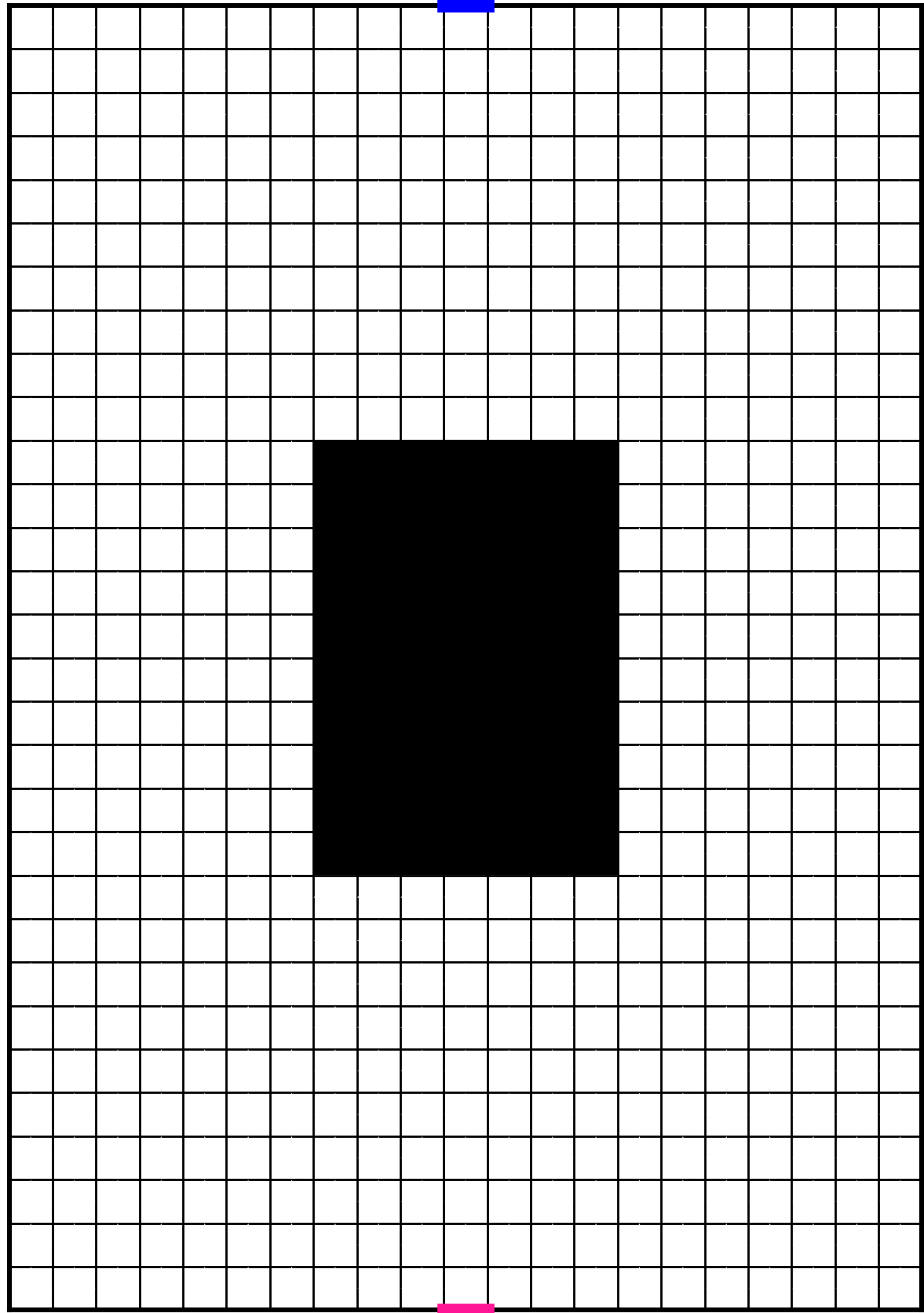
Our environment will be a rectangular gridworld, as shown in the figure below. The width will be 21 pixels, and the height will be 30 pixels. The agent always starts at the bottom center pixel, and tries to get to the target at the top center pixel. On each time step, the agent can only move to one of the four adjacent pixels. Therefore, the action set is of size 4. The agent fully knows its position, which comprises the state. If the agent attempts to move into a wall, then it stays in its current position without moving. The gridworld also contains a non-traversable area of width 7 and height 10 pixels, in the middle, colored in black. The goal of the agent is to find the fastest way to get from the starting position to the target pixel at the top center. To substantiate this goal we give a constant negative reward of -1 for each action the agent takes.

Before we start visualizing policies, let’s think about the optimal policies of the environment, forgetting about entropy. First of all, since the environment is deterministic, we can talk about optimal trajectories. Here are three different optimal trajectories:

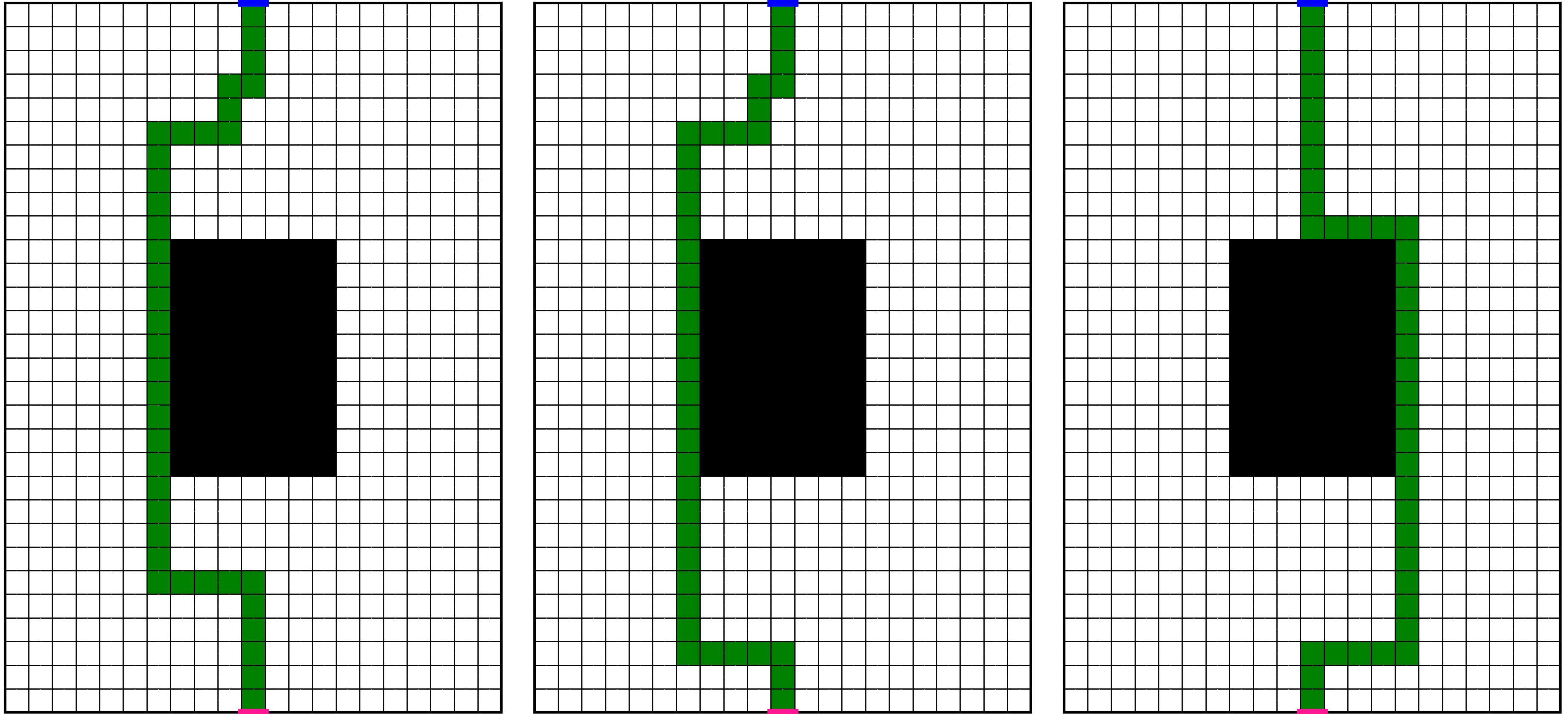
We can see that there are many more optimal trajectories. All other trajectories with the same length, which take us from the initial position to the target pixel, are equally optimal. The number of optimal trajectories is large since our environment posses symmetries, for example: in almost all states, the sequence of actions LEFT,UP gives an identical outcome as the sequence UP,LEFT. Having multiple optimal trajectories means that we have multiple deterministic optimal policies, and this in turn means that we have infinitely many optimal non-deterministic policies. Take any mixture of optimal deterministic policies, with any mixture weights (which can depend on the state), and you get a non-deterministic policy which is also optimal (to make this statement more accurate, we need to consider deterministic policies which are optimal for all states, even for states which have 0 probability of ever being visited when starting from the initial state and following the deterministic policy and environment).

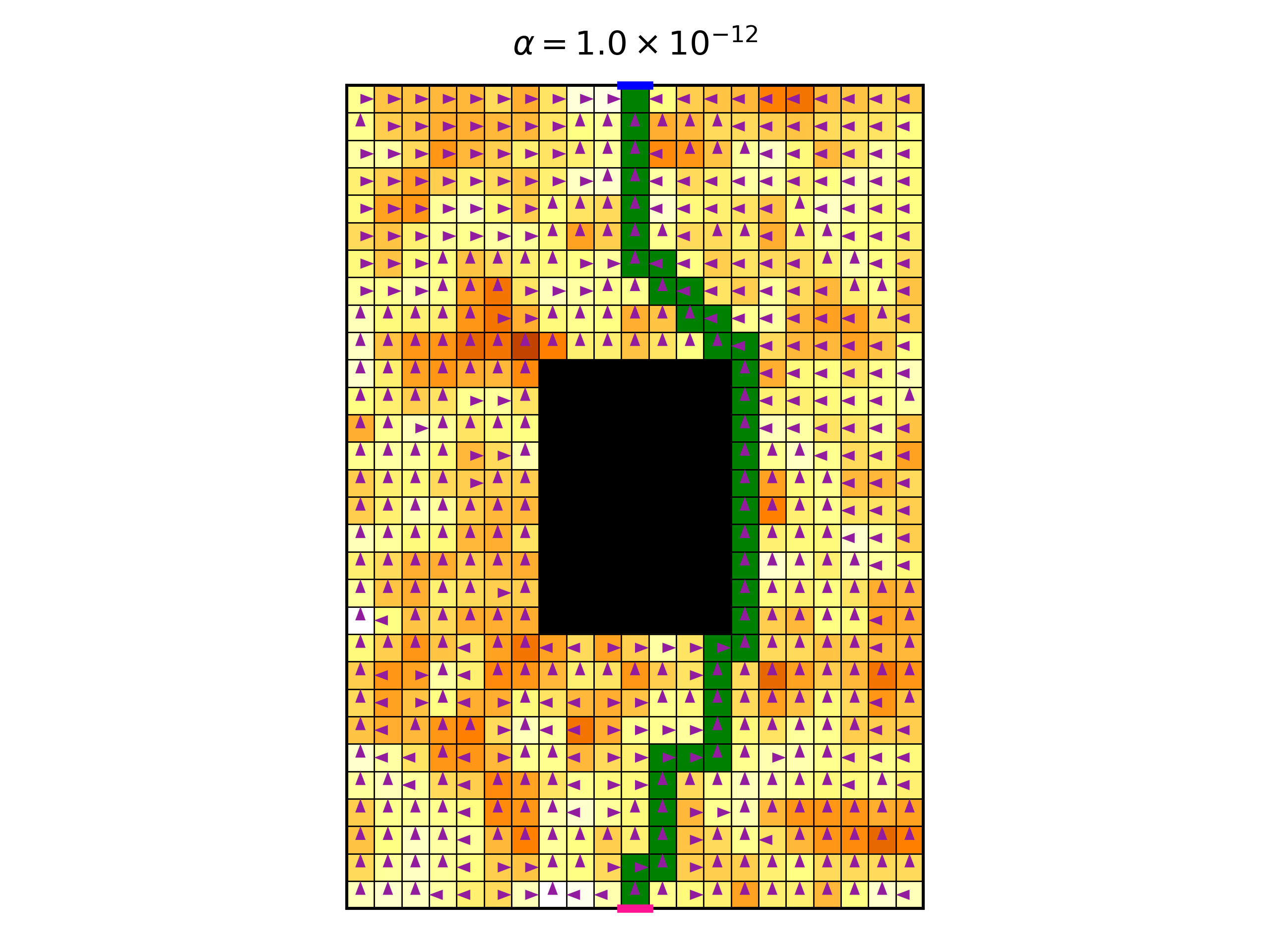
An interesting question is: Among all optimal policies, which policy will we obtain using the policy iteration explained above, in the limit \(\alpha \rightarrow 0\), where the entropy is not important? To test this, we take the value of \(\alpha=10^{-12}\) , and apply the policy iterations until convergence. Here is the resulting optimal policy:

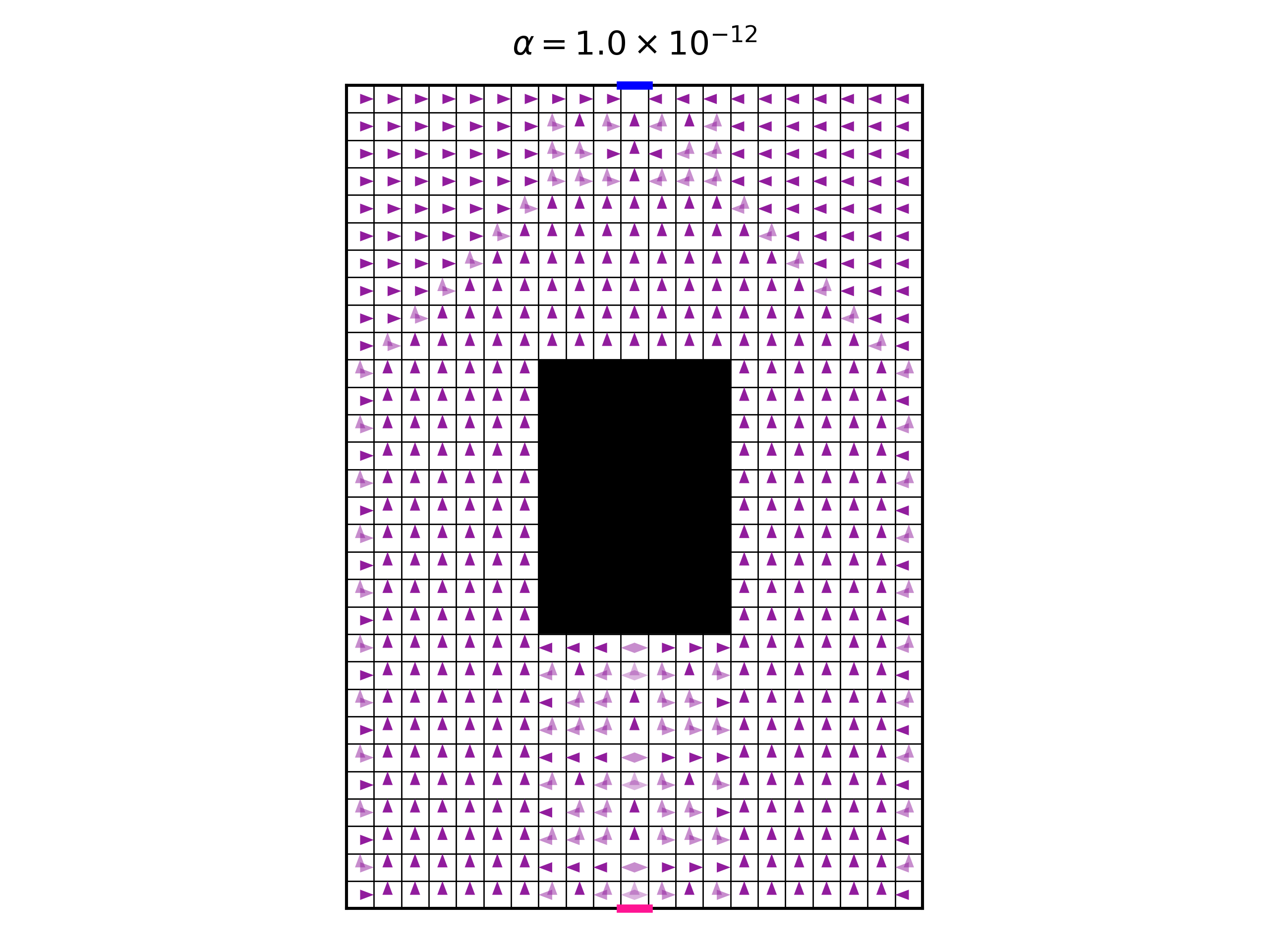
First, let’s explain what this figure shows. It shows the entire policy. On each pixel, there are four arrows, representing the four allowed actions. The color intensity of the arrow represent the probability of the corresponding action under the policy. When an arrow does not show, this means that it has zero probability. The darker the arrow is, the higher the probability it has.

Looking at the policy, we see that it is mostly deterministic. However, in some cases, two or three equally probable actions are allowed. To understand this, we need to remember that the policy is the Gibbs distribution of the Q function, with temperature \(\alpha\). The limit \(\alpha\rightarrow0\) causes the Gibbs distribution to amplify only the single highest value action to the probability of 1, and to attenuate the others to 0. This causes the determinism of the policy. However, in the case of two highest value actions, with equal values, they will both be amplified to 0.5. But any slight numeric difference between the two highest values can make a difference in amplification. Therefore, I believe that the this case is numerically problematic, and we cannot really deduce that the figure represents the true convergence point of the policy iteration (interestingly, running the same optimization with different random seeds, which control the initial value of the Q function, result in the same final policy).

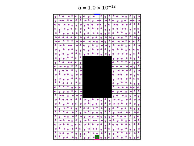
Before we make \(\alpha\) higher, let’s see what happens in the absence of symmetry. To break the symmetry, we change the reward function. Instead of having a constant reward of -1 for each action in all states, we now make the reward depend on the state deterministically (but it still does not depend on the action). We choose some arbitrary reward function, whose reward is in the range [-5, -1]. The following figure shows the environment with the reward function represented as a heat map, where hotter colors represent rewards which are more negative. The figure also shows the optimal policy, for the same small value of \(\alpha=10^{-12}\).

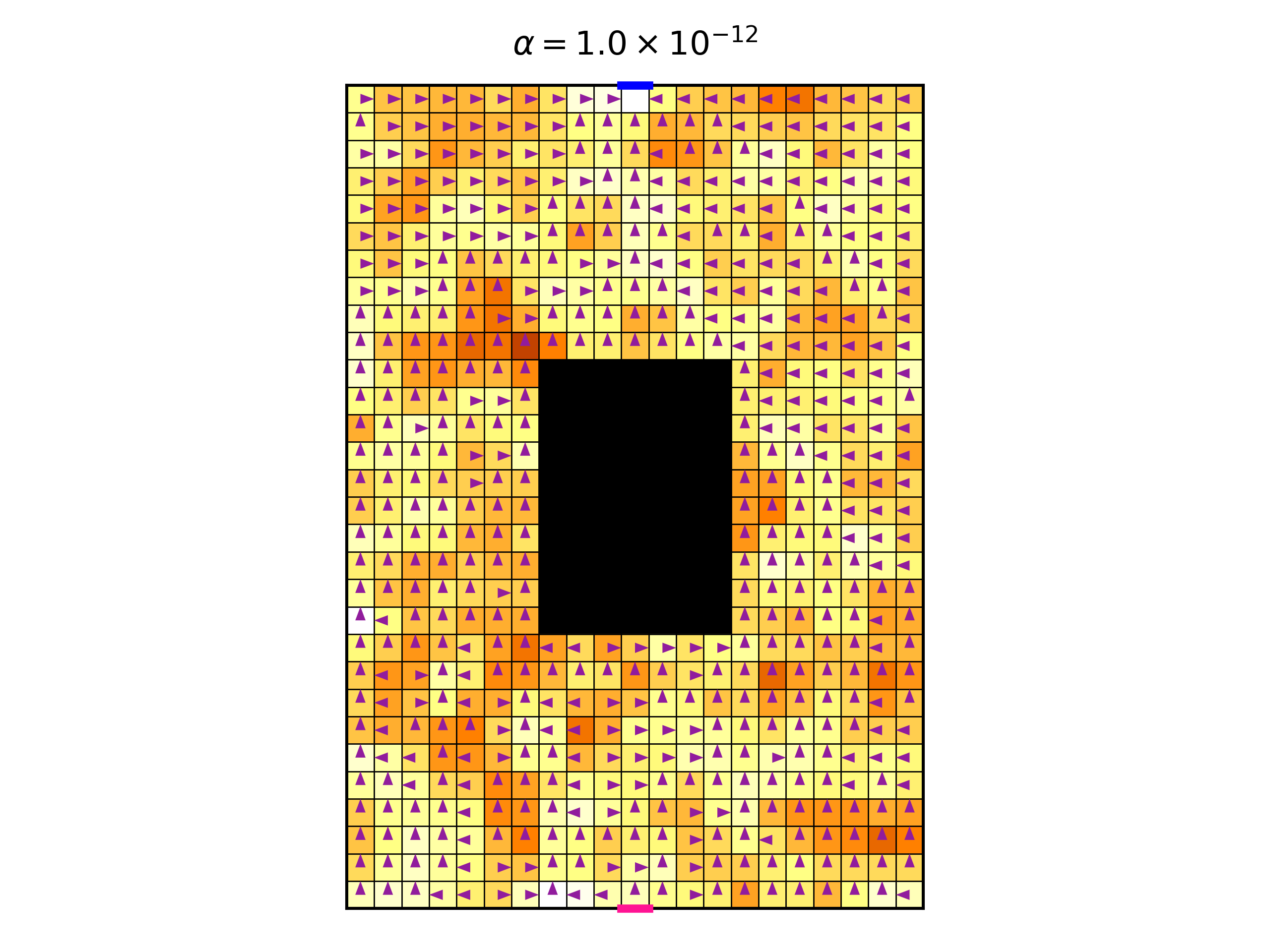
Now we see that we get a fully deterministic policy, not surprisingly. Here is the optimal trajectory:

One last thing, before we start to increase \(\alpha\): It is illuminating to see the policy after each policy iteration step. That is, to view the optimization process of the policy. Here is a video of this process for the symmetrical case, where all rewards are -1, with \(\alpha=10^{-12}\):

The video shows both the policy, and the most likely trajectory induced by the policy, after each policy iteration. Notice how the policy converges most quickly near the target pixel on the top of the gridworld, and from there gradually to the rest of the gridworld. To understand this, we should notice that in the Bellman backup step of the policy iteration, we use the next state’s value. This is not quite true for the final state, which is the target pixel. In this state, there is no next state. Therefore, one single Bellman update is required to get an accurate Q value in this case, and the Q value will not change hereafter. This makes the neighboring pixels to also converge faster, and so on. In fact, what we see here is dynamic programming, and it could be made more efficient if we defer updating pixels which are not near the target pixel, until it is “their turn”.

Ok, so now let’s see what happens when we increase \(\alpha\), thereby giving more importance to the entropy (the SAC paper presents a procedure for optimizing \(\alpha\) using gradients, subject to a constraint on the average entropy. This does not concern this post). We will start with the symmetrical case, where the reward is constant. The following video shows the optimal policy, and the most likely trajectory, as we increase \(\alpha\).

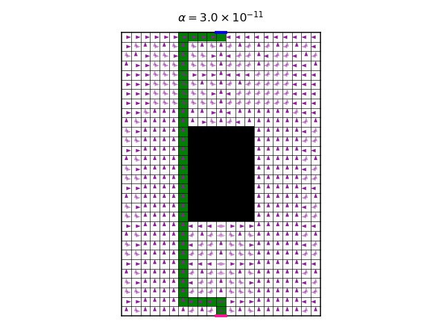
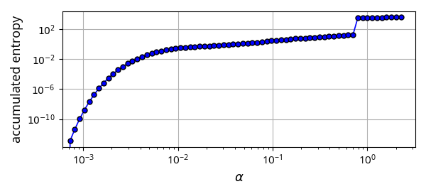
As expected, we see that increasing \(\alpha\) makes the optimal policy less and less deterministic. The final value of \(\alpha\) gives rise to a policy that doesn’t care so much about the reward anymore, only about high entropy. Another interesting observation is that, for a wide range of values of \(\alpha\), the optimal policy is unchanged (note that for each \(\alpha\) we start with a new random initialization of the Q function). Another way to see this is too look at the following graph, which shows the accumulated discounted entropy over the most likely trajectory of the optimal policy for each value of \(\alpha\):

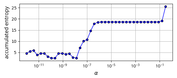
Ignoring the wiggling for small values of \(\alpha\), where results could be less accurate due to numeric errors, we see that the general trend is that entropy increases with \(\alpha\). But we see a range of values of \(\alpha\) , spanning more than 5 orders of magnitude, where the entropy is constant. This might be counter intuitive. We might expect that every small increase in \(\alpha\) will allow the policy to increase its entropy a bit, for the price of a slightly smaller total reward. So why don’t we see this effect for \(\alpha\) in the range \([10^{-6},10^{-1}]\)?

I don’t have a good answer. I suspect that applying reasonings from the physics of phase transitions could help understand this observation. My initial, handwavingly attempt for an explanation is: If we look only at the total reward, without the entropy, then we know that there a subset of deterministic optimal policies. This subset contains many different policies. Now, when the temperature \(\alpha\) is “turned on” (i.e. increased from a zero value to a non-zero value), then all of a sudden the deterministic policies are not good enough, because they have zero entropy. But, by “turning on” the temperature, even if it is still small, then an immediate large increase of entropy can be obtained, by making mixtures of deterministic optimal policies. So, a small increase of temperature causes a large increase in entropy. This large increase “uses-up” all the “budget” of entropy for \(\alpha\) for a long time, until \(\alpha\) becomes large enough again. At some large value of \(\alpha\), mixtures of deterministic policies do not provide enough entropy, and a new optimal policy needs to be found, assigning non-zero probabilities to actions that no deterministic optimal policy would take. Notice that the largest policy entropy possible for each state state is \(\log4\approx1.39\), because we have 4 actions. Therefore, if \(\alpha > 1/1.39\approx0.72\), then \(r+\alpha\mathcal{H}\) can be made positive for all states, since in our case \(r=-1\). This means that for this \(\alpha\), the agent is encouraged to avoid getting to the target pixel, because as time passes, the reward increases. This makes the probable trajectories infinitely long. In the graph, the “turning on” of the temperature occurs at around \(\alpha\approx10^{-7}\) (smaller values of \(\alpha\) might be numerically less reliable), and the “budget” of entropy lasts until \(\alpha\approx10^{-1}\).

My vague explanation asserts that the symmetries play an important role, because it is these symmetries that gives rise to the multitude of optimal deterministic policies. It is therefore interesting to check what happens in the non-symmetrical case, where we use a non-constant reward. So first, let’s look at the video of the optimal policy per \(\alpha\):

And here is the corresponding graph of the accumulated discounted entropy over the most likely trajectory of the optimal policy for each value of \(\alpha\):

The graph shows a more gradual change of entropy as we increase \(\alpha\), which is on par with the theory I suggested above. There is a jump in entropy for \(\alpha\approx0.7\), which is where the entropy becomes more dominant than the reward. This is the point where the trajectories become infinitely long, and their total is in fact the sum of an infinite discounted convergent series.

Looking at the video above, the changes in policy seem quite minuscule as we increase \(\alpha\), I’m not sure why. They only become significant when \(\alpha\approx0.7\), where we observe an interesting pattern where the policy starts to change at the bottom end of the gridworld.

One last interesting exercise is to try and understand an optimal policy. Let’s look at the symmetrical case, with \(\alpha=10^{-3}\). Here is the optimal policy:

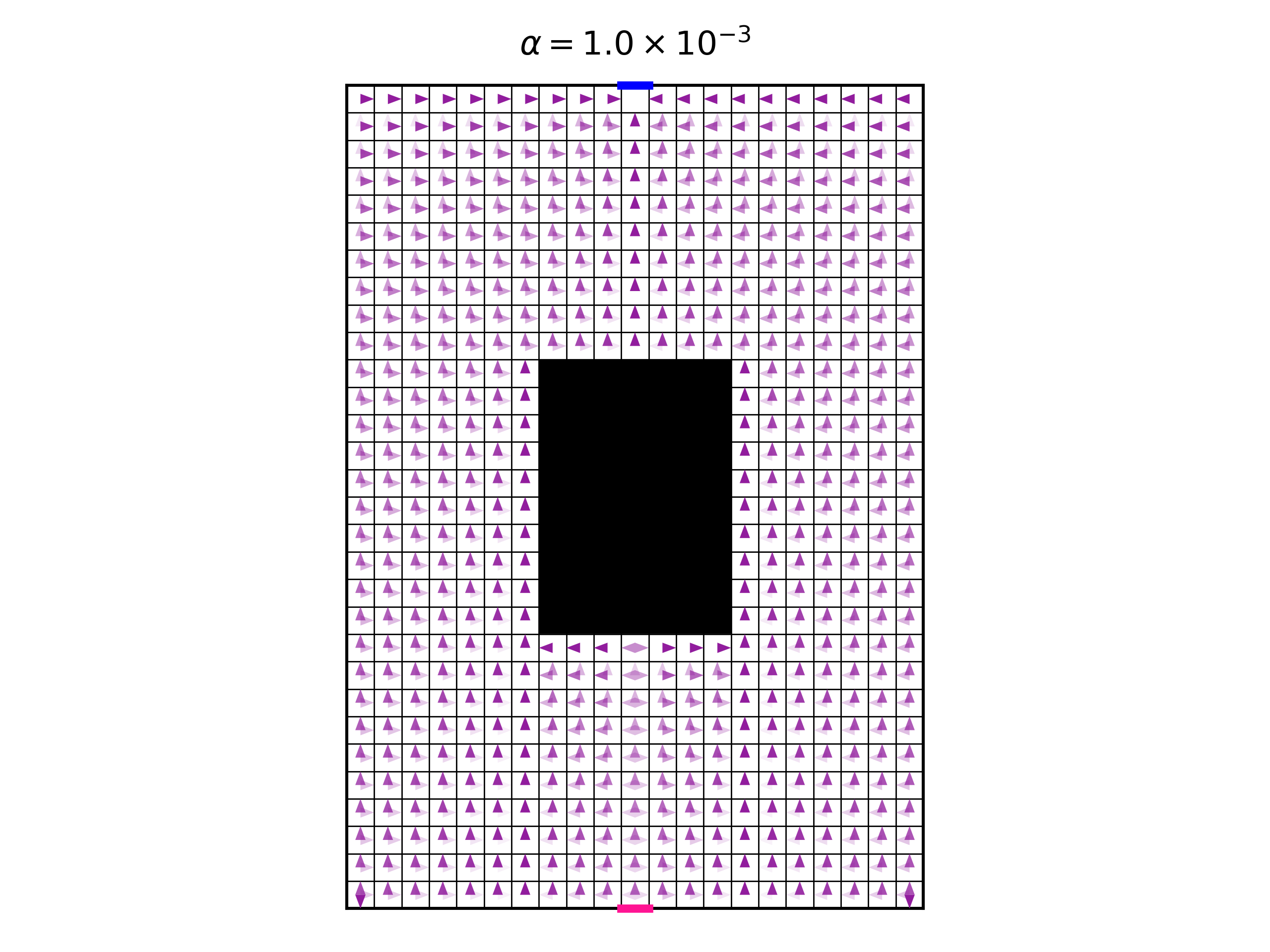
And here, we zoom into one part of it:

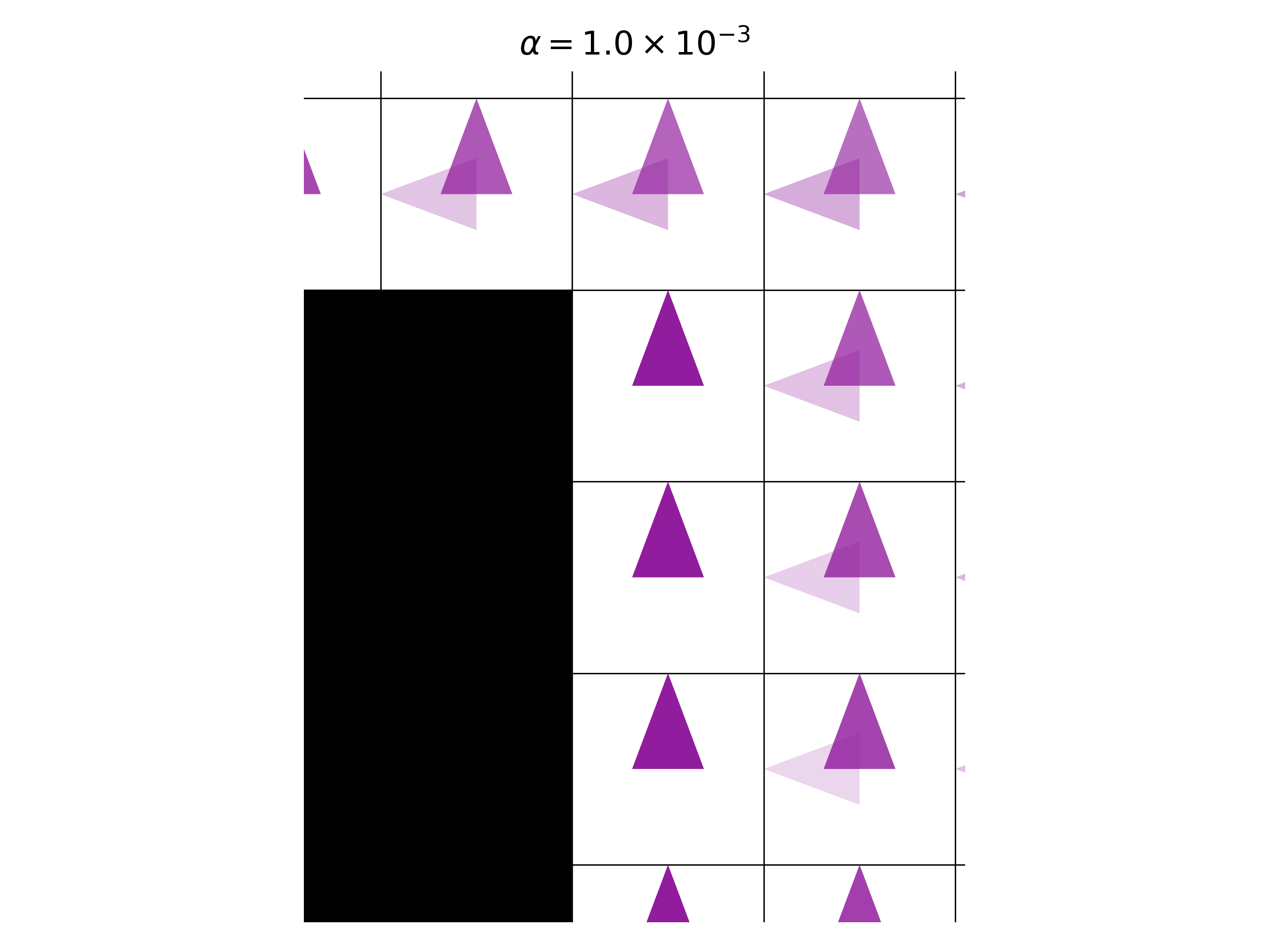
We see that in the column just to the right of the black zone, the policy always makes the deterministic decision of UP. The reason is that, as we explained above, the policy is a mixture of optimal deterministic policies, and all of them take the same actions in these positions. What about the column one step further to the right? We see that here the policy does not take deterministic actions, and it is a mixture of the two possible actions allowed by optimal deterministic policies. But the mixture is not with equal weight. The action UP has higher probability then the action LEFT. How can this be explained? Wouldn’t we get a higher entropy for the uniform distribution over the two actions? Sure, we would get a higher entropy, but this would be a greedy policy. In RL, we care about a cumulative return, not a greedy one. And in this case, if we made the probability for LEFT higher, then we would make the agent more likely to move to the position where the action is a deterministic UP and has zero entropy.

The code used to create optimal policies is here.